Efficiency in Coding

Transcript

We can start to understand the concept of efficiency in computer code and algorithms by comparing it to fuel efficiency in cars. If you’ve ever looked into buying a car, one of the things to consider is a car’s fuel efficiency. How many miles does it get per gallon of gas? Is the number different for city driving versus highway driving? There will probably be a different answer for each car you’re considering.

Another example would be if you managed a team of graphic designers, and had to distribute tasks among them. When choosing a designer, you might take into account how much time and effort each person puts into a task–AKA, how how efficiently a designer completes a task. These factors probably vary across your team.

We can evaluate code in a similar fashion. Like cars or designers, efficiency can vary. Four different lines of code might all complete the same task, but do so in a different amount of time, or using a different amount of memory (or energy).

But there are a lot of different ways to talk about the efficiency of our code. Does efficiency mean the code executes under a certain number of seconds for an average input size? Or, does efficiency mean the code only requires a given amount of RAM before getting an “out of memory” error?

For the most part, software developers are worried about how well their code performs as their input gets bigger and bigger. What if you were trying to find the largest value in an array that’s 10 elements long? What if it were 1,000, or 1,000,000 elements long? By tracking the performance of an algorithm over a variety of input sizes, we can begin to understand how the speed of search changes over time.

end of transcript

Understanding the “Worst Case Scenario”

Let’s look at our car example again. You’ve bought your dream car and immediately take it out for a joyride–an extended joyride. You look at your fuel meter and discover you’re down to your last gallon of gas. The car dealer had told you your car gets about 18 miles per gallon.

You ask Siri where the nearest gas station is, and she tells you it’s 15 miles away. That’s cutting it awfully close, wouldn’t you say?

In the best case scenario, could you get 20 miles per gallon instead of 18? What is the best case scenario (average driving speed, type of road)? What if that last gallon of gas can only get you 14 more miles, based on the type of road you’re on now?

We would describe that last bullet as the worst case scenario.

Inefficiency in Coding: the “Worst Case Scenario”

In coding, we use the idea of the ‘worst case scenario’ to compare the efficiency of different algorithms. That way, we know the code will never perform worse–slower, using up more RAM–than that measurement.

Knowing the best or average case performance of an algorithm is useful, too. But worse case scenario is the standard measure for comparing algorithms.

(If only car dealers made it as clear as that!)

Big O Notation

When it comes to software, we talk about efficiency in terms of Big O Notation. Big O comes from the world of math, where it’s used to describe the relationship between two functions regarding their growth rates.

In software development, Big O focuses on the efficiency of an algorithm as its input increases. It’s used to describe time complexity or space complexity.

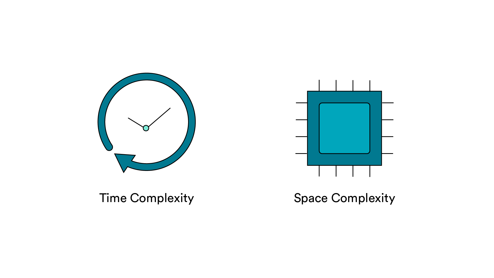
• Time complexity refers to the amount of time an algorithm takes to run.
• Space complexity refers to the amount of memory or RAM an algorithm needs to run.

Let’s take a moment to dive into how time complexity is measured.

Measuring Time Complexity

Time complexity, or the amount of time an algorithm takes to run, is not actually measured in increments of time (seconds, minutes). Instead, we measure time based on the number of basic steps an algorithm needs to execute relative to the size of the dataset it’s working on.

While those steps might look different depending on the context or programming language, something like indexing into an array or adding two numbers together each count as one basic step in Big O.

But: we’re not trying to calculate the exact number of steps a given algorithm takes, either. Big O isn’t about the nitty-gritty details. Instead, it’s a big-picture view on algorithms. It categorizes, at a high level, the differences between algorithms.

If this sounds theoretical, it can actually have pretty big effects on how you build programs and deliver them to users. Take a look!

Why Complexity Matters

Transcript

We were essentially a dating website for private companies and investment banks and mergers and acquisitions people. Forbes called my company “the Tinder of M&A.”

You essentially fill out a dating profile if you’re a company looking to get bought or sold or raise funding. Let’s say that you fill out your corporate dating profile and you want some matches — you want buyers or capital providers to match with you as soon as you fill out the thing.

If you’re matching, if you’re building a recommendation system, there are certain kinds of algorithms that might take a long time to perform. Maybe you click on “Fill out my profile” and you have to wait a few minutes before your matches come in, just because that’s an expensive operation; it’s an expensive problem to solve for. Maybe you want to save all those matches and you just see the saved values — you can’t compute them on the fly.

Knowing that, or knowing that we can do this reasonably quickly, let’s not save them all the time, but we’ll have a loading screen and it’ll take 20 or 30 seconds for these matches to come back. It’s not snappy, but it’s not going to take four hours. It’s an in-between thing.

That’s one time when it came up; when we knew that there was no way to solve this recommender problem that we wanted to give our clients in a super snappy way, but we knew we could do a pretty good job, so we did this weird loading thing. That’s where the CS, or the way we analyzed our algorithm, dovetailed with the user experience.

end of transcript

Knowledge Check

How did algorithmic complexity affect the user experience for Drake’s app?

Click for answer

The time efficiency of the matching algorithm affected how quickly the results loaded for users. Based on the time estimate, Drake added a feature to help users understand what was happening.

Let’s Talk Big O (The Informal Version)

Transcript

Before we get into the technical classes of algorithmic complexity, let’s get familiar with the informal categories we’ll see, using our car analogy once again.

The best, highly efficient algorithms are those zippy little cars that get great gas mileage. They execute in the same amount of time or with the same amount of RAM, no matter the size of the input. Or, they increase a bit as the input increases,1 but then level off.

Pretty good algorithms are your mid-size cars or station wagons. They execute in an amount of time that’s directly proportional to the size of the input. If an input size of 10 elements has an execution time of five seconds, an input of 20 elements has an execution time of 10 seconds.

Inefficient algorithms, on the other hand, have execution time that increases exponentially — or more — as the input increases. They’re your giant, gas-guzzling trucks. Inefficient algorithms vary widely in terms of just how inefficient they can be, but they’re all pretty undesirable compared to the other two groups of algorithms.

end of transcript

Let’s Talk Big O (The Technical Version)

OK, now you know how to describe efficiency in basic terms. Now it’s time to get more technical.

In the rest of the lesson, we’ll cover five “classes of complexity” in algorithms - in other words, breaking down the “highly efficient”, “pretty good”, and “inefficient” groups that we just talked about.

The five classes that we’ll cover are:

Highly Efficient	Pretty Good	Inefficient
Constant complexity	Linear complexity	Quadratic complexity
Logarithmic complexity		Factorial complexity

Constant Complexity: A Highly Efficient Algorithm

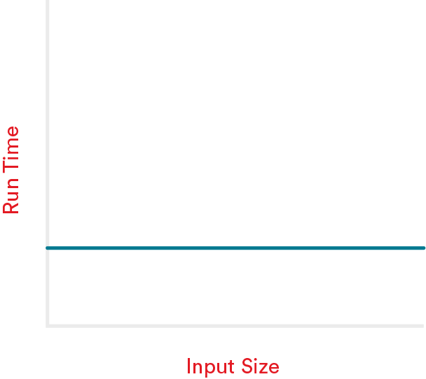
Constant complexity algorithms fall into the “highly efficient” category. They have a constant space (memory usage) and time (number of steps required) complexity, no matter the size of the input.

To understand this type of algorithm, imagine you’re throwing a bag of apples in the trash. This task will always take the same amount of time, no matter if you have 2 or 20 apples in that bag.

In Big O notation, we represent constant complexity algorithms as O(1).

On the next section, we’ll explore two examples of how constant complexity appears in code. As you look at the code, remember: The function will run once, no matter the size of the input. That’s how we get the O(1) notation.

Constant Complexity in Code

So what does an piece of code with O(1) complexity look like? Let’s check out two examples:

Example 1:

function helloWorld(arr) {
  console.log('hello world');
}

Example 2:

let people = {
	instructor: "jimmy",
	student: "doug",
	boss: "shanaz"
	...
}
people.instructor
=> "jimmy"

In both of these examples, the function will run once, no matter what size the input is. That’s how we get the O(1) notation.

Knowledge Check

True or False:

O(1) algorithms are always the fastest type of algorithm, no matter the size of the input.

Click for answer

False. It’s a bit of a trick question! But remember, Big O focuses on the efficiency of an algorithm as its input increases. It’s conceivable that a Constant Complexity algorithm can take longer to run than one with linear or quadratic* complexity--as long as that algorithm takes the same time to run with 1 input or 1,000,000 inputs. If it starts off slow, it’ll always be slow - but the efficiency will be constant.

Linear Complexity: An Algorithm With Pretty Good Efficiency

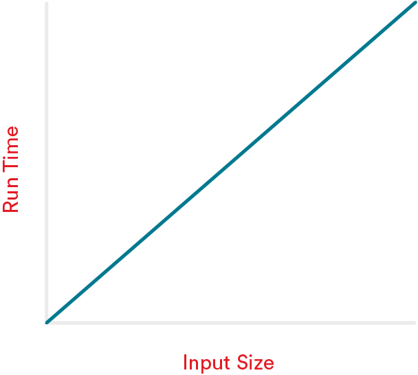
Linear complexity is represented as O(N) in Big O notation. For this type of algorithm, as the input size increases, the processing time increases linearly (one extra input = one more step for the code to perform).

The (N) notation represents just that - the code will run once for every input value.

Remember our apples analogy? This time, instead of throwing out your apples, you decide to peel them to make applesauce. This is a linear task. The amount of time it’ll take you to peel all of them is directly proportional to the number of apples you have in the bag.

The next section has some examples of O(N) in code. In each function, we go through the array and perform an action with each item in it. If we have arr[1], the code will execute once. If we have the array arr[3, 5, 100], the code will run three times. If our array has 1,000 items, the code will execute 1,000 times!

Linear Complexity in Code

Usually, linear complexity means there’s is a loop inside the function or algorithm that iterates over every element in the input size. In plain speak, this means as the input increases, the loop will have to run more and more iterations.

Consider these two functions.

Function 1

function iterate(arr) {
  arr.forEach((item) => console.log(item));
}

Function 2

function iterateLoop(arr) {
  for (let i = 0; i < arr.length; i++) {
    console.log(arr[i]);
  }
}

Knowledge Check

In 2009, an IT company in South Africa was frustrated by their slow internet speed. One employee complained, “It would be faster to transmit our data by carrier pigeon than over the internet!” The company chose to test this claim publicly.

For the test, the company set out to transmit their data from one facility to another — a total of 60 miles. A carrier pigeon delivered a flash drive with the data, while at the same time, the company transmitted the same data through their broadband internet.

The carrier pigeon won. (Nature: 1. Technology: 0.)

How would you represent the speed of the pigeon and the broadband using Big O?

1. The pigeon is O(1) and the internet is O(N).
2. The pigeon is O(N) and the internet is O(1).

Click for answer

Answer #1 is correct. No matter how much data the flash drive contains, the pigeon is going to take about the same amount of time to complete the task every time, which is `O(1)`. The speed at which it takes to transfer the data through the internet, however, greatly depends on how much data is being transferred. The more data, the longer it will take, which is O(N).

Quadratic Complexity: An Inefficient Algorithm

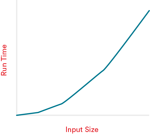
For an input with the size N, quadratically complex algorithms execute N*N times, giving us the Big O notation for this class: O(N^2).

Put another way, these algorithms may have a nested loop, like in this example:

function consoleLogLots(arr) {
  for (let i = 0; i < arr.length; i++) {
    for (let j = 0; j < arr.length; j++) {
      console.log(arr[i], arr[j]);
    }
  }
}

To imagine counting the number of steps, consider that each iteration through the outer loop counts as 1 basic step per element in the input data. Next, in the inner loop, there is a basic step for each element in the input data, but the inner loop runs from beginning to end, for each iteration of the outer loop. We can multiply the number of steps taken in the inner loop by the number of iterations in the outer loop - N*N - or N^2, the notation for this function.

Quadratic Complexity in Code

Looking at our nested loop function:

function consoleLogLots(arr) {
  for (let i = 0; i < arr.length; i++) {
    for (let j = 0; j < arr.length; j++) {
      console.log(arr[i], arr[j]);
    }
  }
}

For the array [1, 3], this function will print:

[1, 1]
[1, 3]
[3, 1]
[3, 3]

For a 2-item array, the code executes 4 times. This scales pretty fast – for an array with 100 items this code will console.log() 10,000 times!

Quadratically complex equations are very inefficient, and should be avoided as much as possible.

Logarithmic Complexity: A Highly Efficient Algorithm

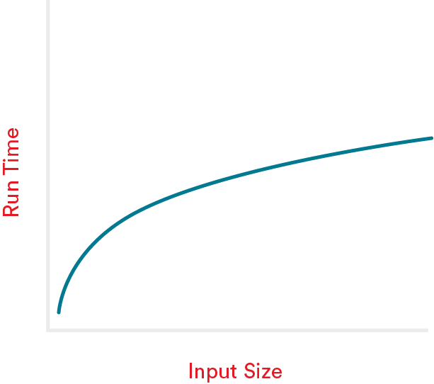
Logarithmic Complexity is represented as O(log (N)). This type of algorithm cuts the problem in half each time. That makes them fast and efficient! And, despite their name, we don’t actually have to calculate logarithms. That’s great news.

Imagine flipping through a phone book to find a someone’s number. You could start at the beginning of the phone book and read every name on every page until it found the name you’re looking for. Sounds awful, right? That’s a linear (O(N)) algorithmic approach.

Instead of reading every single name, it’s much easier to read one random name and flip forward or backward depending on how close that name is to the name you’re looking for. This approach is a logarithmic O(log (N)) algorithm. Much faster!

Logarithmic Complexity in Code

This phone book example is an illustration of binary search, which is a classic O(log(N)) algorithm. In an unsorted array, if we want to find the index of an item with a given value, we have to iterate through it and check if each item is equal to the item we are searching for. However, if we know that we have a sorted array, we can do this a lot more easily!

We’ll spend a lot more time with this algorithm soon, but as a sneak preview, here’s the binary search algorithm:

function binarySearch(arr, item, first = 0, last = null) {
    if (!last) last = arr.length
    let midpoint = Math.floor((last - first) / 2) + first
    if (arr[midpoint] === item) return midpoint
    if (arr[midpoint] > item) return binarySearch(arr, item, first, midpoint)
    if (arr[midpoint] < item) return binarySearch(arr, item, midpoint, last)
}

Let’s say we want to find the value 5 in arr[1, 3, 5, 7, 9, 11, 13]. The function above would run three times instead of the seven that we would need if we iterated through the entire array!

This logarithmic algorithm is super efficient, because even if we have a million items in our array, on average we will only need to execute the binary search 20 times.

Factorial Complexity: An Inefficient Algorithm

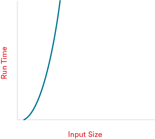
Factorial complexity, represented as 0(N!) should be avoided at all costs. Here’s why.

One example of an O(N!) algorithm is the “bogosort” — aka, the “slow sort.” Why so slow? An array is randomly ordered over and over again until it is correctly sorted. For an array with a length of 10, this sort may have to run up to 3,628,800 times!

Sometimes this complexity category can’t be avoided, but it should raise some red flags.

Comparing Algorithm Classes

Let’s compare the runtimes of the five classes of complexity we covered for a variety of increasing inputs:

			Run Times
Input Size (n)	O(1)	O(logN)	O(N)	O(N^2)	O(N!)
1	1	1	1	1	1
10	1	3	10	100	3628800
40	1	5	40	1600	8.16e+47
80	1	6	80	6400	80!
600	1	9	600	360000	600!
10000	1	13	10,000	100,000,000	10,000!

Visualizing the Difference

Constant Complexity O(1)

Logarithmic Complexity O(log(N))

Linear Complexity O(N)

Quadratic Complexity O(N^2)

Factorial Complexity O(N!)

Drop the Coefficients

Recall that Big O is a relatively high-level way to categorize algorithms. We’re not getting into the nitty-gritty of precisely how much time it takes for an algorithm to run, but instead, looking at its overall efficiency as an input size increases.

For this reason, it’s conventional in Big O to drop coefficients, constants, and other less significant terms when describing an algorithm’s complexity. We’re less worried about the exact runtime of an algorithm and more about the broad category into which it falls (linear complexity, quadratic complexity, etc.).

Take a look at these functions:

Example 1:

function iter(arr) {
  // Big-O: N
  arr.forEach((item) => console.log(item));
  arr.forEach((item) => console.log(item));
  console.log('hello world');
}

Example 2:

function helloWorld() {
  // Big-O: 1
  console.log('hello world');
  console.log('hello world');
}

At first glance, you might think they have complexities of O(2N + 1) and O(2), respectively. However, in order to keep things simple, we can drop the coefficients. The time complexities are still linear and constant — and that’s all that matters for Big O!

Knowledge Check

What’s the complexity of searching for a value in an unsorted array?

1. O(1)
2. O(N)
3. O(N^2)
4. O(log(N))
5. O(N!)

Click for answer

O(N) You’re starting at Index 0 and going up — as a worst case, you might have to look through every item (N Items) to find the value.

Knowledge Check

What’s the complexity of searching for a value in a sorted array?

1. O(1)
2. O(N)
3. O(N^2)
4. O(logN)
5. O!

Click for answer

O(logN) You can run binary search, which cuts the runtime in half at each step, which gives you logarithmic complexity.

---

Why Big O?

Transcript

No matter what car dealership you visit, fuel efficiency is talked about in basically the same way. If you’re in the United States, it’s always expressed in miles per gallon - two standard units of measure. In you’re in Europe, it’s expressed in liters per kilometer. This consistent language makes it easier for car shoppers to compare and contrast models.

In the same way, developers want to be able to compare the algorithms at their disposal and make an informed choice about which to use in a given scenario. If you need your algorithm to process information very quickly, you might trade off a higher space complexity for a lower time complexity.

Big O can also help us categorize problems into different types of complexity. If we are trying to find a given number in an unsorted array, that problem can best be solved in linear time, no matter what algorithm we use. If we are searching a sorted array, the time improves to logarithmic time, no matter the algorithm we use. By knowing the complexity of a given problem, we can pick the algorithm that will best fit with it.

end of transcript

Let’s Talk About Interviews

Big O is a popular technical interview subject because of just how fundamental it is to the way that we talk about algorithms. Interviewers want to make sure that you understand the difference between efficiency and inefficiency so that you aren’t writing code that takes excessive memory or energy to run.

You could be asked to look at an algorithm, determine its Big O complexity, and give your reasoning. If so, keep the following considerations in mind:

• Does the function have to go through an entire list? If so, there’s an N in that Big O class somewhere.
• Are there nested loops? That might give you O(N^2) (or worse).
• Does the function break the list into smaller chunks? You could have O(log(N)).
• Is the amount of work the same, regardless of the size of the data set? You might have O(1).

You could also be asked to describe how a given function could be rewritten more efficiently. As you’ve probably realized, most functions can be written in multiple ways. Big O helps you understand the most efficient way to write functions.