Visualize It

Imagine that you’re a teacher grading your students’ essays. You’re dividing the essays into piles based on their letter grade: A, B, C, D, or F.

In order to sort the essays by grade, you don’t need to compare one essay to another. Maybe the essays were evenly distributed across each letter grade, or maybe every student got a B — it doesn’t matter! You just need to know each essay’s grade in order to put it in the correct pile. That’s how distribution sort works.

Knowledge Check

After you divide your students’ essays by letter grade, you have 10 essays in the B pile with these grades:

[87, 84, 89, 84, 82, 85, 80, 88, 81, 84]

Now, you want to sort all of those essays by their numerical grade. What type of sort would you use?

1. Comparison Sort
2. Distribution Sort

Click for answer

Comparison Sort A comparison sort makes more sense here, as you’d be comparing one grade to another in order to sort them. Distribution sorts are often used in conjunction with comparison sorts.

Types of Distribution Sorts

In this lesson, we’ll cover two common implementations of the distribution sort method: bucket sort and radix sort.

• Bucket sort is a lot like the essay-grading scenario we just explored. It sorts elements into buckets based on their value and then uses another method to sort the elements within those bins. It can be used for integers or strings.
• Radix sort operates in basically the same way as bucket sort but is only used for integers.

Makin’ Buckets

For both bucket and radix sorts, the most important thing you need to decide is: How many buckets should there be?

The answer? It depends on your data set. If you were sorting a lot of elements alphabetically, 26 buckets (one per letter) might work. Or, if you were sorting numbers with radix sort, 10 buckets (one for each digit) could be a good starting place.

A general rule of thumb: If there’s no one obvious way to create your buckets, use the square root of the number of items you’re sorting. So, if you have an array of 100 elements, 10 buckets would be appropriate.

When to Use Bucket Sort

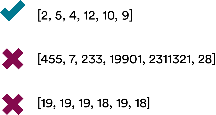
Bucket and radix sorts are most useful when you have a relatively dense range of numbers. “Dense” just means that the values in your starting array are relatively close together.

However, you don’t want your data set to be too dense. If your data set is very dense (i.e., its values are all the same or very similar), it would all be sorted into one bucket. This makes bucket sort’s efficiency a slow O(N^2)!

How Bucket Sort Works

Here’s the general idea of how bucket sort works:

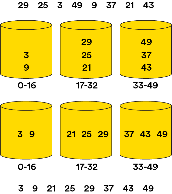
1. Start with your initial array; let’s say we have [29, 25, 3, 49, 9, 37, 21, 43].
2. Set up an array of initially empty “buckets.” Because this array contains eight elements, we’ll use three buckets to start: Bucket 1, 0-16; Bucket 2, 17-32; Bucket 3, 33-49.
3. Go over the original array and scatter each object in its bucket: Bucket 1, [3, 9]; Bucket 2, [29, 25, 21]; Bucket 3, [49, 37, 43].
4. Sort each bucket: Bucket 1, [3, 9]; Bucket 2, [21, 25, 29]; Bucket 3, [37, 43, 49].
5. Gather: Go through the buckets sequentially and gather everything back into the original single array.

Knowledge Check

Can you guess bucket sort’s Big O space efficiency?

1. O(1)
2. O(N)
3. O(log(N))

Click for answer

O(N) Because bucket sort creates an entirely new array for the sorted values, it has O(N) space efficiency. This should sound like another algorithm we met recently — merge sort!

How Radix Sort Works

Without getting too deep into the weeds, radix sort operates by looking at the individual digits in a set of numbers. Radix starts at either the beginning of a number (the most significant digit approach) or the end of a number (the least significant digit approach) and works through each digit until it’s reached the end and the values are sorted.

Let’s use the least significant digit approach on this unsorted array: [270, 65, 30, 603, 3, 84]. (If you’re thinking that this array isn’t dense enough for radix sort, you’re correct! We’re just using it here for the purpose of illustration.)

1. We’ll start by sorting the values based on their least significant digit — the ones’ place: [270, 30, 603, 3, 84, 65].
2. Next, we’ll sort this array based on the next digit — the tens’ place: [603, 3, 30, 65, 270, 84]. (Note that if a number doesn’t have anything in the tens’ place, like 3, we act like there’s a 0 there.)
3. Finally, we’ll sort based on the most significant digit — the hundreds’ place: [3, 30, 65, 84, 270, 603].

Like magic, right?

Knowledge Check

You removed the top earners’ salaries from the database, so you’re left with this data set. It’s denser now and perfect for bucket sort!

Salary
66,000
71,000
59,000
52,000
68,000
55,000

How many buckets would you use to sort this data?

• 6
• 1
• 2
• 5

Click for answer

2 Because there are six values in this database, two buckets would work well here. (You could also make the argument that three buckets would work, as the square root of six is 2.449.)

Let’s Talk About Interviews

You’re more likely to be asked about bubble, insertion, merge, or quick sorts in an interview than bucket or radix sorts. But it’s important to know how distribution sorts work, how they differ from comparison sorts, and the basics of bucket and radix sorts.

To get a better sense of how these algorithms work, use this visualization tool!

• Bucket sort visualization
• Radix sort visualization

Because we won’t discuss how to implement radix sort in code, you can read more about it here.